We’re given this C source code:

1
2
3
4
5
6
7
8

#include <unistd.h>

int main(int argc, long **argv) {
  if(*argv[1] * 0x1064deadbeef4601u == 0xd1038d2e07b42569u){
    execl("/bin/sh", "sh", 0);
  }
  return 0;
}

If we can provide the correct number in *argv[1], passing this conditional, we’ll execute a /bin/sh shell on this suid binary and win. Continue on to see how it was solved.

Something is different in argv

Normally the main function in a C program will look something like int main(int argc, char **argv) where argc is the number of arguments provided, including the program name as argument 0, and char **argv or similarly char *argv[] which is an array of pointers to character arrays (C strings) representing each argument.

The program’s environment variables char **envp, (the third argument to main, which has been left out in this case), and the commandline arguments are loaded into the beginning of the stack area when the program loads.

Let’s say we run this program like this ./level02 one two three four, and have a look at how that area of the stack looks in radare2.

1
2
3
4
5
6
7
8
9
10
11
12
13
14
15
16
17
18
19
20
21
22

$ r2 -d ./level02 one two three four
-- I accidentally the kernel with radare2.

Process with PID 27842 started...
= attach 27842 27842

#  Short binary analysis
[0x564684b24050]> aa
[x] Analyze all flags starting with sym. and entry0 (aa)

# Debug Continue Until main
[0x564684b24050]> dcu sym.main

hit breakpoint at: 564684b24135

#  Analyse Register rdi, first argument to main, normally named argc
[0x564684b24135]> ar rdi
0x00000005

#  Analyse Register rsi, second argument to main, normally named argv
[0x564684b24135]> ar rsi
0x7ffe26db3678

This is the X86_64 calling convention of putting function arguments in order in the registers: rdi, rsi, rdx, rcx, r8, r9 which means main was called essentially like this: main(rdi, rsi), or in this case literally main(5, 0x7ffe26db3678).

Somewhat confusingly this C program types argv differently, this will be important later. So the four arguments we gave, plus the program’s name gives us 5 here, and the stack address 0x7ffe26db3678 will be a pointer, to a pointer, to those argument strings, so let’s look at that now.

1
2
3
4
5
6
7
8
9

#  Print Hex, 0x50 bytes at the address pointed to by rsi
[0x564684b24135]> px 0x50 @ [rsi]

- offset -       0 1  2 3  4 5  6 7  8 9  A B  C D  E F  0123456789ABCDEF
0x7ffe26db5785  2e2f 6c65 7665 6c30 3200 6f6e 6500 7477  ./level02.one.tw
0x7ffe26db5795  6f00 7468 7265 6500 666f 7572 004c 535f  o.three.four.LS_
0x7ffe26db57a5  434f 4c4f 5253 3d72 733d 303a 6469 3d30  COLORS=rs=0:di=0
0x7ffe26db57b5  313b 3334 3a6c 6e3d 3031 3b33 363a 6d68  1;34:ln=01;36:mh
0x7ffe26db57c5  3d30 303a 7069 3d34 303b 3333 3a73 6f3d  =00:pi=40;33:so=

We can see here the following arguments, ./level02, one, two, three, and four, each separated by a 0x00 null character to terminate the string. After that we have a similar situation for environment variables, LS_COLORS=... shown here, which we don’t care about.

An Argument String is Not an Integer

Remembering that char **argv and char *argv[] mean essentially the same thing in C, let’s find out what happens when that is changed to long **argv.

In the normal course of things char *argv[] holds an array of char * which are C strings as shown above. In this program we have long **argv which essentially means a pointer to an array of pointers to long. Confusing?

Basically what this is going to do is force a string entered on the commandline to be interpreted as a type of 64-bit signed int called a long. It’s going to force the bytes in a string to be interpreted as a 64-bit number, which we’ll subsequently do some math on. Computers don’t care about data types, and in C we can take any pointer to some bytes and say, consider the following bytes as this type.

Let’s have some fun, and convert an 8 character string into a 64-bit integer, a long as this program is doing.

1
2
3
4
5
6
7
8
9
10
11
12

#include <stdio.h>

int main(int argc, char **argv){

  char *string = "ABCDEFGH";
  long *integer = (long *)string;

  printf("sizeof(long) = %d\n", sizeof(long));
  printf("%p\n", *integer);

  return 0;
}

Giving the output:

1
2
3

$ ./string_to_int
sizeof(long) = 8
0x4847464544434241

We can see, because X86_64 is little endian, A = 0x41, B = 0x42, and so on, is now backwards, and represents a fairly large 64-bit number.

Finding the Correct Number for argv[1]

Since we now understand how a commandline string can represent a number, let’s find that number so we can pass the following condition:

1

  if(*argv[1] * 0x1064deadbeef4601u == 0xd1038d2e07b42569u)

This should be as simple as taking this equation and rearranging it terms of x:

1
2

x * 0x1064deadbeef4601 = 0xd1038d2e07b42569
x = 0xd1038d2e07b42569 / 0x1064deadbeef4601

This works out to x = 12, and it’s wrong. This is because we’re mixing regular algebra with integer division and disregarding that integers on the computer have a finite range due to bit depth, and wrap around when they exceed the resolution of bits used.

Now let’s say we have, for example 8-bit unsigned integers and multiply 99 * 5 = 495. The maximum value of of an 8-bit unsigned integer is 2^8 - 1 = 255, and this is too high. Counting 0, we have a total of 256 distinct values.

In order to find out how this expression will actually work out on the CPU we can say instead 99 * 5 mod 2^8 = 239, which is the answer you would get for 8-bits after it wraps around. We’ll use that next for our 64-bit values.

I’m going to use Wolfram Alpha to solve for x, because I don’t know offhand how to do algebra involving modulus. First we’ll convert the large 64-bit hex into decimal. I very much like hex, but Wolfram Alpha doesn’t. Boo to that.

1
2

0x1064deadbeef4601u = 1181313840091973121
0xd1038d2e07b42569u = 15061036807694329193

Then entering this equation into Wolfram to solve for x:

1
2
3
4

mod(1181313840091973121 * x, 2^64) = 15061036807694329193

Solution is this set of linear equations:
x = 18446744073709551616 * n + 8319100071223652201  forall n

This will give a valid solution for any n, because of the cyclic nature of integer overflows, so let’s just pick n = 1.

1
2
3

n = 1
x = 18446744073709551616 * n + 8319100071223652201
=> 26765844144933203817

We now have one of an infinite amount of solutions, but we have a problem, this number is too large to fit into 64-bits. How can we tell how many bits a number needs to be represented? The base 2 logarithm of a number will let us know exactly how many bits are needed.

1
2
3
4
5
6
7
8
9
10
11
12

x = 26765844144933203817
Math.log2(x)
=> 64.53702695614811

#  Requires just slightly more than 64-bits.
#  Wrap it back into 64-bit range, gives us a 63 bit number, which is fine
wrapped = x % (2**64)
=> 8319100071223652201

#  Now fits into 62-ish bits, good.
Math.log2(wrapped)
=> 62.85113317948744

Looks like we should have just picked n = 0 and saved ourselves some time. I figured as much, but we got to show off the log2 thing, so whatever. I’m interested in knowing if we can solve this with values of n < 0, but not that interested at the moment :)

Next we need to check that 8319100071223652201 is the number we’re looking for by multiplying it out, this looks like it’s going to be a HUGE number, so we’ll again need to use modulus to wrap it back within 64-bits.

1
2
3
4
5
6
7
8
9
10

8319100071223652201 * 1181313840091973121
=> 9827468051246619677849523421944489321

#  Again wrap it back into 64-bit
(8319100071223652201 * 1181313840091973121) % (2**64)
=> 15061036807694329193

#  Exactly the number that will pass the conditional
0xd1038d2e07b42569
=> 15061036807694329193

Convert our found number to hex

Our number is 8319100071223652201, and in hexadecimal that is 0x7373617034366f69. This looks suspiciously like each byte is an ASCII character value to me, forming an 8 character string, so let’s convert that in radare.

1
2
3
4
5
6

> ? 0x7373617034366f69
hex     0x7373617034366f69
octal   0715633027006415467551
int64   8319100071223652201
string  "io64pass"
binary  0b0111001101110011011000010111000000110100001101100110111101101001

Looks like we have found the commandline argument that will get us our suid shell, io64pass so let’s try it out.

1
2
3
4
5
6
7
8

$ ls -lah level02
-rwsr-xr-x 1 root root 17K Jan  7 01:02 level02

$ ./level02 io64pass
# whoami
root
# id
uid=0(root) gid=0(root) groups=0(root)

It looks like a CrackMe, or capture the flag exercise. The x86 assembly is clearly a virtual machine, and I assumed the block of text on the right would be a binary that runs on that virtual machine. I call the machine, for lack of a better name, Dan32, because as I later found out, it is a 32-bit virtual machine, and originates from Denmark.

The block of text on the right is base64 encoded, which is easy enough to to convert back into a binary file, but since it is an image, we can’t directly get at that block in a text format without doing some kind of optical character recognition. We can guess it is base64 encoded by the characters used, and really after you’ve seen a lot of base64, you can usually spot it pretty easily.

I tried a few online OCR services, which did not work, and since I had invested almost no time into this, I was ready to say the hell with it. I was not about to type all that base64 text into my text editor by hand.

I did end up solving this puzzle and creating tools to reverse engineer it, what follows is a detailed writeup, read on for more.

Note: If you are using a blocker such as Privacy Badger, like I do, I’ve noticed the terminal movie playback embeds from asciinema.org may be blocked by default. If you wish to see those in this post, you’ll have to toggle that domain to allow in your plugin, though you don’t need to accept cookies from that domain for it to work.

Getting the Base64 Text

Staring at it a bit longer, we notice certain characters in the base64 side are bolded, and if we go through and write down each bolded character, it spells out some nonsense MzJoYWNrZXI1NTd6amt6aS5vbmlvbgo..

I thought, since we are looking at a massive bunch of base64, that maybe this was also base64 encoded. We can use a tool called rax2 which is a part of Radare2 in order to decode it like this:

1
2

$ rax2 -D MzJoYWNrZXI1NTd6amt6aS5vbmlvbgo.
32hacker557zjkzi.onion

It’s a vanity .onion address on the TOR network. The site, which unfortunately is not online anymore, has downloads for both the assembly listing, and the base64, saving us from needing to worry about how to get those characters into our computer by hand.

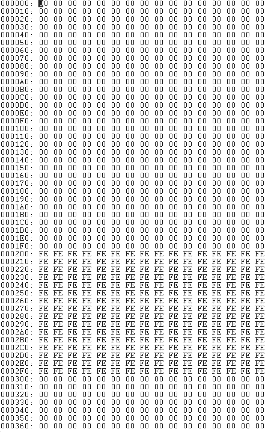
My approach to these sorts of files, that might be malicious or not, is usually to use hexdump or a hex editor program to look at them before going any further. After doing this to the base64 file, I notice that it is full of ANSI terminal escape sequences, and that these ones are for positioning text at (x,y) coordinates, setting bolding etc. This is because if you were to cat the file to your terminal, it would reproduce the formatting seen in the image, with the question mark and all, which is pretty cute, and are actually required to put the text in the right order to be decoded.

Before I cat this to my terminal, I wrote a script to check each of the ANSI escape sequences to make sure they were only positional and style commands, and nothing weird or malicious. They turned out alright, so I printed it to my terminal and copy pasted the text into a file. Then I wrote another script to remove the end of line hyphens, join it all together, and base64 decode it, resulting in a binary file that I named disk.img

You can find the complete source code for all of the Radare2 plugins I wrote to solve this on my github.

The Virtual Machine

The provided x86 assembly for the virtual machine is bare bones, but it tells us everything we need to know to run this binary. The label OP_TABLE points to an enumeration of each opcode the VM supports, and the order, so we know the numeric value of the that op.

Some more information we learn from the given asm is

• There are at least 64 registers in this machine
• It must be a 32-bit machine
• %define REG(r) [REGS + r * 4] Registers are 32-bits wide
• %define PTR(p) [MEM + p] It requires some read/write memory space
• lea esi [DISK + esi] It requires some read/write space to act as a disk
• mov eax, [OP_TABLE + eax * 4] Every opcode is 4 bytes wide
• cmov is the only way to do conditionals

Even after learning all that information, it’s incomplete, some of the opcodes are not given implementations, such as write, in, div, and the various sized load.x, store.x, and nor, to name a few. So we’ll need to look at what’s given, and implement those ourselves.

My Philosophy of Reversing

Here’s where a major part of my reverse engineering philosophy comes in, I don’t as a rule like to run random binaries given to me, especially in malware/crackme situations. If I take the VM’s assembly listing, complete the missing implementations, and run the mystery binary disk.img, I have literally no idea what it is capable of at this point. Worst case scenario is that binary knows about flaw in the given virtual machine, and exploits it for a VM escape onto my host system and starts doing shit.

I’m heavy on the static analysis side, but at this point I don’t have any debugger, or analysis tools that even understand this made up computer architecture. What I want to do, is use Radare2 to reverse engineer the binary, so I’m going to need to teach Radare2 about this file format, computer architecture, invent a textural assembly language, and so on. And that’s the real fun of this challenge for me, honestly, so that’s what I did. Radare2 allows you to write plugins to extend it, so it can understand any CPU, real or imagined, and simulate its running through ESIL (Evaluable Strings Intermediate Language).

Radare2 Plugins

The first Radare2 plugin to write, is the asm plugin. This plugin takes the 32-bit machine level opcodes and fills in a structure with information about that opcode, its arguments, and it provides a textual representation for viewing a disassembly listing.

In order to do this, we’ll write a plugin in C. The asm plugin’s main function has the following prototype

1

static int disassemble(RAsm *a, RAsmOp *op, ut8 *buf, ut64 len);

The parameters to disassemble are:

• RAsm *a is the current assembler context
• RAsmOp *op is the structure we need to fill in
• ut8 *buf are the opcode bytes we are disassembling
• ut64 len is the length of buf

The important fields of RAsmOp to fill in here, are buf_asm which holds the textual representation of the disassembled opcode, and size, the size of the opcode.

Looking at the provided x86 assembly code, we can see how to dismantle a 32-bit opcode into its constituent parts, remember all opcodes are 4 bytes long or 32-bits.

1
2
3
4
5
6
7
8
9
10
11
12
13
14

mov ebp, edx
shr ebp, 21
and ebp, 77o
mov esi, edx
shr esi, 15
and esi, 77o
mov edi, edx
shr edi, 9
and edi, 77o

mov eax, edx
shr eax, 27
mov eax, [OP_TABLE + eax * 4]
jmp eax

Becomes

1
2
3
4
5
6
7
8
9
10
11
12

#define SIX_BIT 077

//  Cast 4 bytes from buf to a unsigned 32 bit value
ut32 dword = *(ut32*)buf;

//  32 - 27 leaves a 5-bit opcode
ut8 op_index = (dword >> 27);

//  Extract 3 6-bit arguments using the SIX_BIT mask
ut8 edi = (dword >> 9 ) & SIX_BIT;
ut8 esi = (dword >> 15) & SIX_BIT;
ut8 ebp = (dword >> 21) & SIX_BIT;

Next, for convenience, we make a lookup table that maps 0 to 63 to the corresponding register name. I happen to know from the future, that r62 is the stack pointer, and r63 is the instruction pointer, but I didn’t know this at the time. It makes reading the disassembly a lot easier though once we know this.

1
2
3
4
5
6
7
8
9
10
11
12

static const struct {
    char *name;
} regs[] = {
  { "r00" }, { "r01"  }, { "r02" }, { "r03" }, { "r04" }, { "r05" }, { "r06" }, { "r07" },
  { "r08" }, { "r09"  }, { "r10" }, { "r11" }, { "r12" }, { "r13" }, { "r14" }, { "r15" },
  { "r16" }, { "r17"  }, { "r18" }, { "r19" }, { "r20" }, { "r21" }, { "r22" }, { "r23" },
  { "r24" }, { "r25"  }, { "r26" }, { "r27" }, { "r28" }, { "r29" }, { "r30" }, { "r31" },
  { "r32" }, { "r33"  }, { "r34" }, { "r35" }, { "r36" }, { "r37" }, { "r38" }, { "r39" },
  { "r40" }, { "r41"  }, { "r42" }, { "r43" }, { "r44" }, { "r45" }, { "r46" }, { "r47" },
  { "r48" }, { "r49"  }, { "r50" }, { "r51" }, { "r52" }, { "r53" }, { "r54" }, { "r55" },
  { "r56" }, { "r57"  }, { "r58" }, { "r59" }, { "r60" }, { "r61" }, { "esp" }, { "eip" }
};

Since in the disassembly output we’re going to be referencing things by register name a lot, I grab the textual names for each argument as well.

1
2
3

char *edi_reg = regs[edi].name;
char *esi_reg = regs[esi].name;
char *ebp_reg = regs[ebp].name;

What follows in the disassemble function is a switch statement on op_index, where we just need to fill in the op size and the textual representation of the opcode itself. So I’ll show a few of those here, you can see the full source of these plugins here

1
2
3
4

  case 11:
    snprintf(op->buf_asm, R_ASM_BUFSIZE, "nor %s, %s, %s", ebp_reg, esi_reg, edi_reg);
    op->size = 4;
    break;

So for example the nor instruction, which wasn’t provided in the image, just uses snprintf to write out our human readable disassembly, and sets the op->size = 4. This ends up producing something like nor r21, r57, r57.

Quickly taking a look at another example, movi is the move immediate value instruction, and looks like this:

1
2
3
4
5
6
7
8
9
10
11

case 16:
  eax = dword;
  ecx = dword;
  eax >>= 5;
  eax &= 0xffff;
  ecx &= 037;
  eax <<= (ecx & 0xff);

  snprintf(op->buf_asm, R_ASM_BUFSIZE, "movi %s, 0x%0x", ebp_reg, eax);
  op->size = 4;
  break;

Notice op->size = 4 for all instructions, and setting op->size = -1 indicates an invalid operation. The above movi instruction actually encodes an immediate value directly into the opcode itself. This is the only instruction which does this, all other instructions must move values into a register to operate on them. Again, this is a straight translation from from the given x86 asm.

Other instructions had to be put together just following the pattern that was set out for us. For example, div, mul, nor all work the same as the given mul opcode. All said, it is not a lot of work to get a fully functioning disassembler going in Radare2.

Here is the last part of the plugin, where we hook our code up by setting callbacks, and some information:

1
2
3
4
5
6
7
8
9
10
11
12
13

RAsmPlugin r_asm_plugin_dan32 = {
  .name = "dan32",
  .author = "safiire@irkenkitties.com",
  .license = "None",
  .desc = "Dan32 disassembler",
  .arch = "dan32",
  .bits = 32,
  .init = NULL,
  .fini = NULL,
  .disassemble = &disassemble,
  .modify = NULL,
  .assemble = NULL,
};

And here’s the result, a nice looking assembly readout that we can use to start reversing the binary.

Radare Analysis Plugin

With the above plugin we can now see human readable disassembly of the binary, but Radare doesn’t have enough information about this architecture yet to allow us to step through the program and simulate it like you would in a debugger. And you can’t yet perform static analysis like you would get with IDA. Radare supports about one zillion architectures already, but since this CPU was probably invented just for this challenge, we’ll have to add support ourselves.

Radare’s answer to this is ESIL, (Evaluable Strings Intermediate Language), providing a register profile for the CPU, and using those to create an analysis plugin. An analysis plugin expects us to implement a function like this, to set the register profile.

1
2
3
4
5
6
7
8
9
10
11
12
13
14
15
16
17
18

static int set_reg_profile(RAnal *anal) {
  const char *p =
  "=A0  r03\n"
  "=A1  r04\n"
  "=A2  r05\n"
  "=LR  r59\n"
  "=PC  r63\n"
  "=SP  r62\n"
  "gpr r00 .32   0 0\n gpr r01 .32   4 0\n gpr r02 .32 ... etc"
  "gpr r08 .32  32 0\n gpr r09 .32  36 0\n gpr r10 .32 ..."
  "gpr r16 .32  64 0\n gpr r17 .32  68 0\n gpr r18 .32 ..."
  "gpr r24 .32  96 0\n gpr r25 .32 100 0\n gpr r26 .32 ..."
  "gpr r32 .32 128 0\n gpr r33 .32 132 0\n gpr r34 .32 ..."
  "gpr r40 .32 160 0\n gpr r41 .32 164 0\n gpr r42 .32 ..."
  "gpr r48 .32 192 0\n gpr r49 .32 196 0\n gpr r50 .32 ..."
  "gpr r56 .32 224 0\n gpr r57 .32 228 0\n gpr r58 .32 ..."
  return r_reg_set_profile_string(anal->reg, p);
}

Here we specify all 64 general purpose registers in the machine, and also give aliases to registers that have special meaning. The format is gpr <registername> .<size in bits> <offset>.

With this we can create a register file containing registers of various sizes, which can overlap. For example in x86, we can specify register gpr ax .16 0, but also specify the high and low bytes as gpr ah .8 8 and gpr al .8 0.

Dan32 doesn’t have overlapping registers, or high and low register access by name, so we don’t need to do this.

Some register aliases are A0, A1, A2, which are for arguments that are passed to functions via register, which is pretty common in this binary. LR is the link register, which like on an ARM CPU holds the return address of a function, PC, is the instruction pointer, and SP is the stack pointer, so I’ve filled those in after having gotten some experience with the binary’s two calling conventions.

The next task for the analysis plugin is to create ESIL for each and every instruction supported by the CPU. There are not many instructions so this didn’t take very long.

The plugin must implement an analysis function with the following prototype, which looks extremely similar to the asm plugin function:

1

static int dan32_anal_op(RAnal *anal, RAnalOp *op, ut64 addr, const ut8 *data, int len);

Here, we’re asked to fill in more information about the opcode in the given RAnalOp *op parameter, it looks something like this:

1
2
3
4
5
6
7
8
9
10
11
12
13

struct RAnalOp {
  id       // I use the opcode index
  esil     // A string containing ESIL
  size     // Size of opcode, this is always 4 in dan32
  nopcode  // No idea, other plugins set this to 1
  addr     // Address this opcode is at
  jump     // If this opcode jumps somewhere, the address
  fail     // Where to jump on failure condition
  ptr      // Pointer to the primary data we're working with
  val      // Value of the primary data we're working with
  type     // enum of types such as R_ANAL_OP_TYPE_CJMP for conditional jump
  family   // enum of type family such as R_ANAL_OP_FAMILY_IO for I/O
}

All of these are pretty important for proper analysis, but the most important, so that we can simulate this binary inside radare2, without running it on the untrusted VM we were given, is the ESIL. Here is an example of ESIL for movi, the move immediate value instruction:

1
2
3
4
5

movi r57, 0x41

; becomes

0x41,r57,=

ESIL is a stack machine, turing complete, so it is able to represent the instructions for any CPU, it is like a ridiculous sort of microcode almost. A more complicated instruction cmov, the conditional move instruction, looks like this:

1
2
3
4
5

cmov eip, r57 if r23

;  becomes

r23,?,{,r57,eip,=,}

So after each instruction is codified by type and given an ESIL representation, we’re done. If you are interested in how ESIL works, here’s the docs. I’ve written some pretty crazy ESIL for the disk sector read/write code, and stack machines are not my favourite, but they work :) Here is some of the longest ESIL I wrote for one opcode. It reads 512 bytes from a numbered disk sector, into a given memory address.

1
2
3
4
5
6
7
8
9
10
11
12
13
14

read [r57], sector(r21)

;  becomes

0x0,r40,=,
0x200,r21,*,
0x200000,+,
r40,+,
[8],
r57,r40,+,
=[8],
0x8,r40,+=,
0x200,r40,==,!,
?{,3,GOTO,}

Disassembling the binary in Radare2

Ok, so now we’re all set to get a disassembly view of this binary, we’ll just load it up in Radare2, hit play to see how it goes.

“Wrong Endianness”. Now, there are a few things going on here, so let’s look at the first instruction: movi r00, 0x78200. I don’t want to get to bogged down in the details, but I know from the future, that register r00 is like the zero register on a MIPS system, it always contains the value 0, and so here writing 0x78200 to that register, is effectively a no-op, and we’ll see why that’s done in the next part.

Next up we have movi eip, 0x14. There are no jump instructions in this opcode set, and unlike x86, you can write to the instruction pointer register to get a jump. Interestingly, jumping to 0x14 is not a multiple of 4, and so we’re jumping out of alignment, which is why we’re seeing the disassembler isn’t able to interpret a few instructions after that at first.

When we get to the address 0x14, we end up at series of instructions that loads immediates, and then uses out to print them out to the display.

1
2
3
4
5
6
7
8
9
10
11

0x00000014  e00a2087    movi r57, 'W'
0x00000018  000020cf    out r57
0x0000001c  21072087    movi r57, 'r'
0x00000020  000020cf    out r57
0x00000024  e00d2087    movi r57, 'o'
0x00000028  000020cf    out r57
0x0000002c  e1062087    movi r57, 'n'
0x00000030  000020cf    out r57
0x00000034  e00c2087    movi r57, 'g'
0x00000038  000020cf    out r57
0x0000003c  25002087    movi r57, ' '

A little bit of radare knowledge, the immediate values were displayed as hex to begin with, so I wrote a little radare expression to hint to it that those immediates are actually string or char values using the ahi command, which stands for “analyse hint immediate”.

Radare2 is terse as hell, and you get very used to it, and probably, maybe, start loving it. The expression below basically creates a range from the current address, denoted as $$, to $$ + 17 * 8 with a step of 8 bytes. The @@= functions as an iterator, which runs the command ahi s on each address in the range, telling radare the immediate values are character values.

1

ahi s @@=`?s $$ $$+17*8 8`

Anyway, the real problem is we’re interpreting the binary as little endian, when it’s actually big endian. So we can just go back to our plugin and fix that pretty simply in the disassemble function by reversing the bytes, and setting the endian properly.

1
2
3
4
5
6
7
8
9
10
11
12
13
14
15
16
17
18
19

//  Decode the op
ut8 big_end[4];
big_end[0] = buf[3];
big_end[1] = buf[2];
big_end[2] = buf[1];
big_end[3] = buf[0];

ut32 dword = *(ut32*)big_end;
ut8 op_index = (dword >> 27);       // 5-bit opcode

// ...

RAsmPlugin r_asm_plugin_dan32 = {
  // ...

  .endian = R_SYS_ENDIAN_BIG,

  // ...
};

Correct Endian

Back to the entrypoint of our binary, what was once a no-op, when read backwards, jumps us past all the “Wrong Endian” stuff, and begins displaying the binary properly so we can reverse it.

The opcode 87e00180 when read in big endian jumps us with movi eip, 0xc, and another jump movi eip, 0xa8, bringing us finally to some actual code.

1
2
3
4
5
6
7

0x000000a8   movi r20, 0xc0
0x000000ac   movi r21, 0x14c
0x000000b0   movi r22, 0xbe
0x000000b4   store.b [r22], r00
0x000000b8   read [r00], sector(r00)
0x000000bc   goto r21
;  print "Disk read error!"

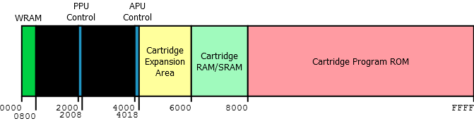
This is the first in a series of tricks and tests that the binary performs on the virtual machine itself to make sure it is implemented properly. With the use of a bin plugin for dan32, which I’m not going to bore you with here but is available on GitHub with the rest of the code, I’ve tried to setup a memory layout that would be familiar for someone like myself who works with ELF or PE files. Here is that layout.

1
2
3
4
5
6
7

00  0x00000000 |#-------------------------| 0x0000092b  2.3K mrwx .text
01  0x0000092c |#-------------------------| 0x00000b79   589 mrw- .bss
02* 0x00000c00 |#-------------------------| 0x00007503 26.3K mrw- .encrypted
03  0x000ffc00 |------------#-------------| 0x00100000    1K mrw- .stack
04  0x00200000 |-------------------------#| 0x00207503 29.3K mrw- .diskrom
05  0x00100000 |------------#############-| 0x001f0000  960K -rwx esil.ram
=>  0x00001dc0 |--------------------------| 0x00001ec0

Remembering the DISK address that was mentioned in the x86 assembly VM, which is meant to represent a readable writeable disk area from which the program is loaded. This area stores disk.img in the .diskrom section at address 0x200000. I probably shouldn’t have called it a diskrom, since you can write to it, but I didn’t know it was going to be written to at the time, so it’s too late now. I actually believed it was going to be something like a game cartridge rom at first, but oh well.

The code is executed from the .text section, with entrypoint 0x0, and we have a .bss section which contains some initialized data that is used in the program. The read and write instructions are used to copy data from the disk into memory by 0x200 byte sectors.

So the trick here, is that at 0xb4 we are writing from r00, which always contains zero to address 0xbe, which is altering an instruction. Then, if your read instruction works properly this is immediately corrected by reloading the entire first sector from .diskrom back into memory, undoing the damage. If your read instruction is not working, you will be greeted by the text “Disk read error!” and the program will halt.

Notice how the analysis plugin is working, showing beautiful ascii arrows that point to the destinations of our jumps. When the zero is written to address 0xbe, it modifies the instruction, and we see the control flow is taking us directly towards “Disk read error” and a halt. The read immediately fixes this and the control flow updates.

The Next Test

Next we move on to 0x14c, which is an area of the binary that sets up the stack pointer, and reads the rest of the program from .diskrom one sector at a time.

I guess here we can get our first look at how dan32 goes about things.

1
2
3
4
5
6
7
8

;-- fcn_read_other_sectors:
0x0000014c      add r61, eip, r00
0x00000150      movi r57, 0x4
0x00000154      nor r57, r57, r57
0x00000158      add r61, r61, r57
0x0000015c      movi r57, 0x1
0x00000160      add r61, r61, r57
0x00000164      movi esp, sym.stack_end

Here’s some things to take note of right off the bat:

• There is no subtraction instruction
• There is no concept of signed numbers
• We can still have negative numbers using 2’s complement
• There are no other bitwise logical operations besides NOR
• NOR is universal, and can construct any other gate
• There is no direct way to move one register into another one, so addition + 0 is used
• nor(a, a) flips all the bits of a
• nor(a, a) is equivalent to -(a + 1) in 2’s complement
• r00 is a hardware zero register
• r57 is used as a temporary register

There’s a few patterns we see using NOR throughout this binary. Above we want to save the instruction pointer to r61, and then subtract 4 from it. This is done many times in this binary like this:

1
2
3
4
5
6

add r61, eip, r00     ;  r61 = eip
movi r57, 0x4         ;  r57 = 4
nor r57, r57, r57     ;  r57 = -5
add r67, r61, r57     ;  r61 = r61 - 5
movi r57, 0x1         ;  r57 = 1
add r61, r61, r57     ;  r61 = r61 + 1

This is a roundabout way of just saying r61 = eip - 4, but that’s what we’re dealing with here :)

The next test the binary performs on the virtual machine, is to test the div instruction. Since this instruction was not provided in the x86 assembly code, it is to ensure we’ve got the argument order right, and we’re not allowing division by zero. If we’ve done it wrong, we’re sent off to some code that prints “ALU Malfunction (DIV)” and halts the program.

By the way, these symbols such as fcn.alu_malfunction_div, fcn.main, and so on, were added by me while reversing the binary to make it more clear what is going on.

1
2
3
4
5
6
7

nor r20, r00, r00                       ; r20 = -1
div r20, r00, r20                       ; r20 = 0 / -1
movi r57, fcn.alu_malfunction_div       ;
add r57, r57, r00                       ; does nothing
cmov eip, r57 if r20                    ; if(r20) goto fcn.alu_malfunction_div
movi r57, fcn.main                      ;
goto r57                                ; goto main()

That’s also our first look at conditionals in dan32. There are no compare instructions, there is no zero flag, and no conditional jumps like jne, as you find in other instruction sets.

An interesting side note I guess, is that there is no real compare instruction in x86 either, the cmp instruction on that processor is actually an alias for subtracting the two values. When they are equal, since a - a = 0, this sets the zero flag, which is what instructions like jne are conditional on.

The Main Function

Now that the Radare plugins are working, let’s have a look around the binary, simulate it a bit, and look around. This is loading a project file where I’ve already reversed the entire binary, but gives a good idea of how it’s working.

Here’s where we start getting some idea of what this binary is up to, and finally get to see some proper functions such as print(), scan(), memcmp() and things like that implemented.

1
2
3
4
5
6

;-- fcn.main:
0x0000028c      movi r03, str.password
0x00000290      movi r57, 0x8
0x00000294      add r59, eip, r57
0x00000298      movi r57, fcn.print
0x0000029c      goto r57

First up, radare has identified a string “Password: “, and helpfully renamed its address as the symbol str.password for us. Here we can see one of the two calling conventions in action. This one is a lot like fastcall, where we load the first few arguments of a function into registers r03, r04, r05, and end up with our return value in r01.

Remember I identified r59 as the link register, and that is used as our return value. So here, the calling convention is to calculate the return address, eip + 8, two instructions away, and store it into r59, we then load the address of the print function fcn.print into a temp register, and jump there.

Throughout the binary, r57 is always used as a temporary register. There are others such as r20, r21 which are always used as counters or array indices. In fact, this assembly code is so consistent in the way it does things and which registers it uses, that I wonder if it was emitted by a machine, or written by hand by someone who is just awesome.

Now that we know our arguments, our return address, and where we’re going, that about fully describes this calling convention. There is also a stack based calling convention like you would find on x86 32-bit, which I may write about later.

The Print Function

So don’t worry I’m not going to bore you to death by literally explaining every function, but this print one is a fairly simple example to start with.

1
2
3
4
5
6
7
8
9
10
11
12
13
14
15
16
17
18
19
20
21
22
23

;-- fcn.print:

;  Initialize r20 to 0 as an array index
add r20, r00, r00
movi r57, lbl.head
goto r57

lbl.body:
   ;  Output the character in r21
   out r21
   ;  r20 += 1
   movi r57, 0x1
   add r20, r20, r57

lbl.head:
   ;  r21 = r03[r20]
   load.b r21, [r03 + r20]
   movi r57, lbl.body
   add r57, r57, r00

;  return if r21 == 0
cmov eip, r57 if r21
goto r59

This function is simple, but normally to reverse a difficult function, I will slowly replace elements of the disassembly with C, until I have a C function. In this case, we’d have a for loop:

1
2
3
4
5

void print(char *r03){
  for(r20 = 0; r03[r20] != 0; r20++){
    out r03[r20]
  }
}

The Purpose of the Program

I’ve kept from mentioning the actual purpose of this program for way too much of this article. If written in C, the main function would just about look like the following code. This was figured out by reversing each function in turn, and I got a happy surprise at the end, we’re going to be dealing with encryption.

1
2
3
4
5
6
7
8
9
10
11
12
13
14
15
16
17
18
19
20
21
22
23
24
25
26
27
28
29
30

void main(){
  printf("Password: ");
  chars_read = scan(passphrase_input);

  if(chars_read == 0){
    print_eh_halt();
  }

  print("Initializing Encryption...");
  burn_cpu();

  rc4_key_schedule(key_schedule, passphrase_input, chars_read);
  print("Ok");
  print("Checking Key");
  burn_cpu();

  decrypt(key_schedule, encrypted_test_data, 0x38);
  result = memcmp(encrypted_test_data, correct_decryption, 0x38);

  if(result != 0){
    print_bad_key_halt();
  }

  print("Ok");

  rc4_key_schedule(key_schedule, passphrase_input, chars_read);
  print("Decrypting Disk Image");

  decrypt_disk();
}

So what’s going on here, is we’re going to do an in-place decryption of the DISK section if we’ve entered the right passphrase.

We’re able to figure all this out, without running this binary at all, through static analysis and a bit of ESIL simulation. I guess the question is how did I know which function was doing the decryption, what actual encryption algorithm was being used, and how I’m going to figure out the passphrase without even running the binary.

The answer to the first question is that I knew I would probably need to find XOR somewhere in this program which would XOR the ciphertext with the key stream, but since we have no XOR instruction, I knew it would need to be created with a group of NOR, which I found pretty easily.

So I spotted that pretty easily, and pinpointed the main decryption routine.

1
2
3
4
5

nor r58, r21, r01
nor r21, r58, r21
nor r57, r58, r01
nor r21, r21, r57
nor r21, r21, r21

The answer to how did I know which encryption algorithm it was, is more funny. I didn’t know which one it was. I had stepped through the key scheduling function a few times, after it prints “Initializing Encryption”, and thought that it was basically key stretching the passphrase. It was only later when I was randomly reading through a writeup on some malware which used RC4 encryption, that I realized what I was looking at the same RC4 key scheduling algorithm.

Cracking the Passphrase

The main encrypted part of the binary was identified by the address that was being passed to the decrypt() function, which was 0xc00. I also previously noticed this while running the binary through the entropy function of the program binwalk. Here is the output from binwalk -E

1
2
3
4
5
6

$ binwalk -E disk.img

DECIMAL       HEXADECIMAL     ENTROPY
--------------------------------------------------------------------------------
0             0x0             Falling entropy edge (0.553052)
3072          0xC00           Rising entropy edge (0.972975)

One of the weaknesses of some encryption schemes, is in how it checks if the passphrase is valid before decryption. Say for example you enter a passphrase on a zip file or something, and the unzip program just blindly decrypts the file without knowing if the password is valid. It’s going to produce total garbage if the passphrase is wrong, and the program won’t have any way of letting you know that you’ve entered the wrong password.

So a common, bad, way to verify the password first, is to have some known ciphertext, plaintext pair that is encrypted using the passphrase right in the binary. You enter the passphrase, it decrypts this small ciphertext, compares it to the known plaintext, and if it’s correct, it says “yay” and moves on to decrypting the rest of the file. If it’s wrong, it says “boo”, and doesn’t decrypt the file into garbage.

This is what’s happening in our dan32 binary. The known ciphertext, plaintext pair is included, meaning we just have to crack that.

Here we can see that before decrypting the DISK section, it tries to decrypt a small 56 byte buffer, and then compares that to a valid string that is included in the program.

1
2
3
4
5
6

  decrypt(key_schedule, encrypted_test_data, 0x38);
  result = memcmp(encrypted_test_data, correct_decryption, 0x38);

  if(result != 0){
    print_bad_key_halt();
  }

Here we can output the short encrypted buffer, and its valid decryption. If the passphrase we give doesn’t decrypt this short buffer correctly, the program will halt. Here I use the px Radare command to do a hexdump of the test ciphertext, and another ps command to print the plaintext string.

1
2
3
4
5
6
7
8
9
10
11

px 0x38 @ sym.another_buffer_i_think

- offset -   0 1  2 3  4 5  6 7  8 9  A B  C D  E F  0123456789ABCDEF
0x00000964  7216 fa85 4c3c d0e4 5905 7954 d203 eb95  r...L<..Y.yT....
0x00000974  1601 e73b 6dc8 642f 742f 5419 aabe ea31  ...;m.d/t/T....1
0x00000984  9306 c9e1 fa65 830f 5118 a727 94ff 9634  .....e..Q..'...4
0x00000994  5af7 4c29 85de 8714                      Z.L)....

ps 0x38 @ 0x0000092c

Another one got caught today, it's all over the papers.

That means in order to crack this passphrase, I only need to figure out how to successfully decrypt this 56 byte buffer, which is something I can do entirely outside of this binary. I decided to reverse the key scheduling and decryption routine, and rewrite it in C so that I could brute force the password quickly outside of this environment, and outside of Radare.

1
2
3
4
5
6
7
8
9
10
11
12
13
14
15
16
17
18
19

//  Here is the reversed RC4 key schedule from Dan32
void rc4_key_schedule(char *key_schedule, char *key_input, int length){
  char *ptr = (key_schedule + 2);
  for(int i = 0; i < 0xff; i++){
    ptr[i] = i;
  }

  int j = 0;
  for(int i = 0; i < 0xff; i++){
    j = (j + ptr[i] + key_input[i % length]) & 0xff;
    char t1, t2;
    t1 = ptr[i];
    t2 = ptr[j];
    ptr[i] = t2;
    ptr[j] = t1;
  }
  key_schedule[0] = 0;
  key_schedule[1] = 0;
}

1
2
3
4
5
6
7
8
9
10
11
12
13
14
15
16
17
18
19
20
21

//  Here is the PRGA from Dan32
char pseudo_random_generation_algorithm(char *key_schedule){
  int i = key_schedule[0];
  int j = key_schedule[1];

  char *s = zero_gap + 2;

  i = (i + 1) & 0xff;
  j = (j + s[i]) & 0xff;

  key_schedule[0] = i;
  key_schedule[1] = j;

  char t1, t2;
  t1 = s[i];
  t2 = s[j];
  s[i] = t2;
  s[j] = t1;

  return s[ (s[i] + s[j]) & 0xff ];
}

And finally the decrypt routine.

1
2
3
4
5
6
7
8

//  RC4 Decrypt from Dan32
void decrypt(char *key_stream, char *cipher_text, int length){
  for(int i = 0; i < length; i++){
    char key = pseudo_random_generation_algorithm(key_stream);

    cipher_text[i] = cipher_text[i] ^ key;
  }
}

I made this into a complete program, that takes a passphrase as argument, and then wrapped it in a short Ruby script that repeatedly tries passwords from a list I have, until the decrypted result matches. This only took about 3 minutes, the passphrase ended up being agent This was lucky, because it could have been a lot harder if it wasn’t a simple word, I would have needed to use hashcat or something a bit more sophisticated. There are also flaws with RC4 itself, which directly relate to the problems with WEP, but I didn’t need to go that route.

I can’t really call writing this code a waste of time, since I ended up needing to do it in order to actually identify the algorithm, but there are far easier ways to decrypt RC4 that I could have used, for example, Radare2 comes with a program called rahash2 which can, among about a zillion other things, be used to decrypt RC4.

1
2
3
4
5
6
7
8
9
10
11

$ hexdump -C test.bin

00000000  72 16 fa 85 4c 3c d0 e4  59 05 79 54 d2 03 eb 95  |r...L<..Y.yT....|
00000010  16 01 e7 3b 6d c8 64 2f  74 2f 54 19 aa be ea 31  |...;m.d/t/T....1|
00000020  93 06 c9 e1 fa 65 83 0f  51 18 a7 27 94 ff 96 34  |.....e..Q..'...4|
00000030  5a f7 4c 29 85 de 87 14                           |Z.L)....|
00000038

$ rahash2 -D rc4 -S s:agent test.bin

Another one got caught today, it's all over the papers.

Decrypting the Disk Image

At this point I am thinking I will just dump the high entropy section of the binary from 0xc00 onwards out to a separate file, and decrypt it with rahash2 and be done with it, but when I try this, I end up with unintelligible garbage, that isn’t proper dan32 code, and isn’t anything else I can recognize.

The DISK section is divided into 512 byte sectors, and it turns out they are not decrypted in the order they appear in the file. The order of the pseudorandomly generated keystream matters since it’s a stream cipher, and so that is why I’m getting garbage out. I decided then to just simulate the decryption process within Radare using ESIL, since I put so much work into properly defining each opcode in ESIL, it does simulate the VM perfectly.

The only problem is, that I have not implemented the in and out opcodes for doing IO, so I would be running the program blind, and be unable to enter the passphrase or see printed output.

Fixing the IO Problem

An easy way to avoid writing the in opcode, is for me to simulate the program up until it is about to ask me for a passphrase, stop there, and just write the passphrase into memory at the right address, and skip over the scan() function entirely and continue afterwards, so that’s what I’ve decided to do.

For the out opcode, there is a less hacky solution. I can use ESIL to simulate an interrupt, and attach that interrupt to an external program that will receive the character value to be printed. I wrote a short Ruby script which accepts an argument and prints it to the standard output. And inside Radare2 simulate the binary like this:

1
2
3
4
5
6
7
8
9
10
11
12
13
14
15
16
17
18
19
20
21
22
23
24
25
26
27
28
29

#  Setup ESIL
s 0
aei
aeim
aeip

#  Allow the binary to virtually write into a memory cache
e io.cache = true

#  And attach out.rb as an interrupt handler
e cmd.esil.intr=!./out.rb


#  Advance to right before we call scan to ask for password
aecu 0x000002ac


#  Write the RC4 password into the right place in memory
#  The length is written to the return value register

wz agent @ 0x1200
aer r01 = 0x5


#  Skip over the call to scan(), and continue from there
#  r63 is the instruction pointer

aer r63 = 0x000002b4
aecu 0x000004fc

The Result

This takes a while to complete, so I just went off and did something else. Another thing, not shown here is that the binary often calls functions that just do nothing but waste enormous amounts of time counting, which have no effect on the output. I patched these calls out of the binary so I wouldn’t have to wait 2000 years for it to finish.

Once all is said and done, the binary has completely rewritten the DISK section into yet another binary, and we’re given this message:

1
2
3
4
5
6
7
8
9
10
11
12
13
14
15

$ # Look, I'm an HTTP server now!
$ cat xinetd.conf
service httpd
{
    disable     = no
    socket_type = stream
    protocol    = tcp
    wait        = no
    bind        = 0.0.0.0
    server      = u5emu
    server_args = disk.img
    type        = UNLISTED
    port        = 80
    user        = root
}

I dump the DISK segment into an actual file, and reload that in Radare, and sure enough it has decrypted itself into a webserver written in dan32. I reversed this new binary for a while, and found it contained:

• Embedded html files
• A GIF of Morpheus from the Matrix
• A PNG background file
• Some lzma compressed issues of Phrack Magazine
• The Hacker’s Manifesto, by the Mentor
• Some zlib compressed files
• And the finally, the flag, written in Danish

I used binwalk to extract these from the binary and looked through the contents. I got the flag, so I’m calling this one done. Good experience overall, 10/10 would crack again. I’m so proficient in reading dan32 assembly now, that it’s a shame I’ll probably never have any use for it again, it’s a pretty nice VM.

So I like to take some of my free time and play hacker wargames like smashthestack.org, or reverse engineer crackmes, so I decided to describe my process for solving those types of challanges here.

Crackmes

“Crackmes” are essentially a compiled binary without source code, which asks you for a password or key, you enter the wrong password you lose, you enter the right one and you win and move onto the next. You need to reverse engineer the binary in order to discover the password, and these range from simple to tedious and difficult as the creator of the crackme piles on layers of obfuscation, misdirection, encryption, and anti-debugging techniques to stop you, not to mention you need a good handle on assembly and keeping track of what is in various memory locations during runtime.

Crackme0x00a

We start out simple, and so I start with my simplest techniques. crackme0x00a wants a password:

1
2
3
4

  ./crackme0x00a
  IOLI Crackme Level 0x09
  Password: blah
  Password Incorrect!

So first we think that perhaps the password is simply in the binary, and we can find it by running the program strings on it to list every string in the program. I think it’s safe to say that will work on this one, but I have a more direct approach that I usually take, and that is run the program through ltrace. ltrace outputs all calls to library functions that the program makes, so here we’re looking for something like a call to strcmp

1
2
3
4
5
6
7

  ltrace ./crackme0x00a
  __libc_start_main(0x80484e4, 1, 0xffa24724, 0x8048570, 0x80485e0 <unfinished ...>
  printf("Enter password: ") = 16
  __isoc99_scanf(0x8048651, 0xffa24663, 0x8049ff4, 0x8048591, -1Enter password: blah
  ) = 1
  strcmp("g00dJ0B!", "blah") = 1
  puts("Wrong!"Wrong!) = 7

Simple, we found the call to strcmp the password is g00dJ0B!. You see how we can see each call, with parameters and return value. This was all that was needed to beat this challenge.

Crackme0x00b

Let’s move onto the next one, with the same approach

1
2
3
4
5
6
7

ltrace ./crackme0x00b
__libc_start_main(0x8048494, 1, 0xff82ec54, 0x8048500, 0x8048570 <unfinished ...>
printf("Enter password: ") = 16
__isoc99_scanf(0x80485e1, 0xff82eb4c, 0, 0xf77f249c, 0xff82ebf4Enter password: blah
) = 1
wcscmp(0x804a040, 0xff82eb4c) = 1
puts("Wrong!"Wrong!) = 7

So the difference here is the password is being compared with wcscmp, which has the prototype int wcscmp (const wchar_t* wcs1, const wchar_t* wcs2); It compares wide strings where each char is 16-bit.

On Linux most of the time the code and data sections get loaded around the address 0x08040000, and local variables are stored in the stack, which begins at the top of memory and grows upwards from 0xffffffff.

The arguments to wcscmp are 0x804a040, which I’m guessing is in the initialized data section, and is the secret password, and 0xff82eb4c which ltrace shows is the location on the stack that it wrote our input to.

The trick to this challenge, is that if we were simply to run the strings program on the binary, it would have worked in the previous challenge, but not this one because each character in a wchar_t string is 32-bits long with the most significant bits zeroed out, and terminated by a a 32-bit 0x0000 value.

The quickest way I know to find out the bytes at 0x804a040 is to load the binary into my debugger radare2 and just print it out.

1
2
3
4
5
6

[0x080483e0]> px 64 @0x804a040
- offset -   0 1  2 3  4 5  6 7  8 9  A B  C D  E F  0123456789ABCDEF
0x0804a040  7700 0000 3000 0000 7700 0000 6700 0000  w...0...w...g...
0x0804a050  7200 0000 6500 0000 6100 0000 7400 0000  r...e...a...t...
0x0804a060  0000 0000 4743 433a 2028 5562 756e 7475  ....GCC: (Ubuntu
0x0804a070  2f4c 696e 6172 6f20 342e 362e 312d 3975  /Linaro 4.6.1-9u

The password is w0wgreat.

Crackme0x01

Ok, let’s see what’s new in the next one, and hopefully get to use radare2 some more. First let’s see what happens with ltrace.

1
2
3
4
5
6
7
8
9

ltrace ./crackme0x01
__libc_start_main(0x80483e4, 1, 0xffdd85c4, 0x8048460, 0x80484d0 <unfinished ...>
printf("IOLI Crackme Level 0x01\n"IOLI Crackme Level 0x01) = 24
printf("Password: ") = 10
scanf(0x804854c, 0xffdd8524, 0xf77a6ff4, 0xf7636dd5, 0xf77c8660

Password: blah
) = 0
printf("Invalid Password!\n"Invalid Password!) = 18

So usually I just write in blah for a password, but we can see here that scanf has returned 0 in response to my string. scanf returns the number of things it has parsed according to its format string. So I’m guessing its format string was not "%s" this time as it was before. Maybe it was looking for a number. Let’s load it into r2, dissassemble the main function and find out.

1
2
3
4
5
6
7
8
9
10
11
12
13
14
15
16
17
18
19
20
21
22
23
24
25
26
27
28
29
30
31

╒ (fcn) sym.main 113
│           ; arg int arg_149ah    @ ebp+0x149a
│           ; var int local_4h     @ ebp-0x4
│           0x080483e4      55             push ebp
│           0x080483e5      89e5           mov ebp, esp
│           0x080483e7      83ec18         sub esp, 0x18
│           0x080483ea      83e4f0         and esp, 0xfffffff0
│           0x080483ed      b800000000     mov eax, 0
│           0x080483f2      83c00f         add eax, 0xf
│           0x080483f5      83c00f         add eax, 0xf
│           0x080483f8      c1e804         shr eax, 4
│           0x080483fb      c1e004         shl eax, 4
│           0x080483fe      29c4           sub esp, eax
│           0x08048400      c70424288504.  mov dword [esp], str.IOLI_Crackme_Level_0x01_n
│           0x08048407      e810ffffff     call sym.imp.printf
│           0x0804840c      c70424418504.  mov dword [esp], str.Password:
│           0x08048413      e804ffffff     call sym.imp.printf
│           0x08048418      8d45fc         lea eax, [ebp - local_4h]
│           0x0804841b      89442404       mov dword [esp + 4], eax
│           0x0804841f      c704244c8504.  mov dword [esp], 0x804854c  ; "%d"
│           0x08048426      e8e1feffff     call sym.imp.scanf
│           0x0804842b      817dfc9a1400.  cmp dword [ebp - local_4h], 0x149a
│       ┌─< 0x08048432      740e           je 0x8048442
│       │   0x08048434      c704244f8504.  mov dword [esp], str.Invalid_Password__n
│       │   0x0804843b      e8dcfeffff     call sym.imp.printf
│      ┌──< 0x08048440      eb0c           jmp 0x804844e
│      │└─> 0x08048442      c70424628504.  mov dword [esp], str.Password_OK_:__n
│      │    0x08048449      e8cefeffff     call sym.imp.printf
│      └──> 0x0804844e      b800000000     mov eax, 0
│           0x08048453      c9             leave
╘           0x08048454      c3             ret

So, woo, radare is the best. It has added helpful identifiers for us rather then make us look up a bunch of addresses. For example str.Invalid_Password__n is an identifier standing in for the address of the string `“Invalid Password\n”.

The assembly listing is easy to follow thanks to the analysis radare2 has done, and the symbols it has added for us, it even graphically shows branches and loops.

The first thing to know when you look at the assembly listing of a function created by a compiler, is that there is going to be 3 main sections: the function prologue, the body, and the function epilogue. If you already know this, you will probably want to skip down a little ways.

The Function Prologue

Like I mentioned before, the stack is an area of memory which in Linux begins at 0xffffffff, and grows upwards in memory, and the CPU register esp points to the top of the stack. To get this analogy you have to think of memory as a something like a container that holds plates. The bottom of the container is 0xffffff, the top of it is 0x000000. When you place plates onto the stack over and over, the pile grows upwards. That is pushing things onto the stack.

To remove things from the stack, you “pop” them off of it. You can’t pop a plate out of the middle or the bottom, you can only pop a plate off the top. It is a LIFO stack, last in is first out.

An x86 CPU has push and pop instructions for this, and guess what, compilers don’t use them very much, prefering to instead just do arithmetic on esp or ebp in order to get values from the stack or manipulate its size.

In a running program, we use the stack as a “function call stack”, which is a sequence of “stack frames”, one per function called.

So let’s explain how that’s laid out so we can get back to the crackme. Take this example nested function calls:

1
2
3
4
5
6
7
8
9
10
11

int h(c){
  int d = 10;
  return c + d;
}
int g(b){
  return h(b + 1);
}
int f(a){
  return g(a + 1);
}
f(0);

1
2
3
4
5
6
7
8
9
10

|      10          | Local variable d  (esp) (ebp - 4)
|   0xffffffef     | Saved ebp frame pointer
| h Return Address |
|       2          | Argument to h
|   0xfffffff7     | Saved ebp frame pointer
| g Return Address |
|       1          | Argument to g
|   0xffffffff     | Saved ebp frame pointer
| f Return Address |
|       0          | Argument to f

The calling convention used here is called cdecl, to call a function we put its arguments on the stack in reverse order, and use the call instruction. call automatically pushes the address of the next instruction after it onto the stack, so we will know where to return to after the function call ends.

Once inside the function, space is made to hold the local variables, usually by subtracting the local variables size in bytes from esp, raising the stack up higher, sometimes this size is aligned on a 16 byte boundry by using the and instruction. This is why there is junk data in uninitialized local variables, they just hold whatever garbage happened to be on the stack.

main() like any other function has a prologue.

1
2
3
4
5
6
7
8
9
10

push ebp                 ; Push the previous base pointer to the stack
mov ebp, esp             ; Make our new base pointer the top of the stack.
sub esp, 0x18            ; Increase the stack space by 0x18 bytes
and esp, 0xfffffff0      ; Align the stack to 16 byte boundry.
mov eax, 0               ; eax = 0
add eax, 0xf             ; eax = 0xf
add eax, 0xf             ; eax = 0x1e
shr eax, 4               ; eax = 0x1
shl eax, 4               ; eax = 0x10 A shift right then left also aligns
sub esp, eax             ; Increase stack space by another 0x10 bytes.

So we save the old base pointer (base pointer, frame pointer, same thing) then start subtracting from esp to increase the space for local variables.

It makes space twice, using two different methods for aligning it to a 16-byte boundry. You could ask, why doesn’t it just do this all in one subraction. I have no idea why it does it this way, but I do know that when you compile with optimizations off, the compiler often does redundant things. You might also ask why it reserves so much stack space for the one 32-bit local variable that actually exists in this main function.

Your guess is as good as mine. In the assembly listing we can see that the only local variable used is called local_4h, which is the value at ebp - 0x4, the int sized local variable that scanf parses our input into.

The Function Epilogue

1
2
3

mov eax, 0
leave
ret

The leave instruction is the same as mov esp, ebp pop ebp. This effectively undoes all the stack resizing the prologue did, and then restores the base pointer to what it was before main was called. Yep, there is another hidden function that calls main()

There is a register called eip that holds the address of the current instruction, but you can’t directly assign a value to it except to use a branching instruction or ret. After leave is executed the next thing on the stack is the return address of the caller, ret pops that address into the eip register and execution continues from there.

A function’s return value is always stored in the eax register, so mov eax, 0 is the same as return 0 at the end of main().

Back to scanf

1
2
3
4
5
6

lea eax, [ebp - local_4h]
mov dword [esp + 4], eax
mov dword [esp], 0x804854c  ; "%d"
call sym.imp.scanf
cmp dword [ebp - local_4h], 0x149a
je 0x8048442

The first instruction, lea stands for load effective address, and is good at doing pointer arithmetic, calculating the address of elements inside arrays, and things like that. [ebp - 4] is the address of the local int sized value on the stack we want scanf to write to.

local_4h is just a symbol radare uses to remind us what is in a memory location, and it allows us to rename it if we want, it just equals 4 in this case.

0x804854c is the address of the constant string “%d” located in the data section. So this code is just moving the value 0x804854c to the top of the stack, and the address of our local variable 4 bytes after that in reverse order that scanf takes them, then we call to scanf.

At this point whatever we wrote, if it was a number, will be located at [ebp - 4], and this value is compared with 0x149a, if they are equal we jump to the “you win” screen.

So that solves this crackme, all we need to type for a password is, in decimal 5274.

1
2
3
4

./crackme0x01
IOLI Crackme Level 0x01
Password: 5274
Password OK :)

Crackme0x02

Ok, let’s hope they get a bit harder from here on, and this should go a lot faster without needing to explain the stack, etc.

A quick run shows that ltrace is not going to help us this time, so back into radare we go. I’ve renamed some of the local variable so it will be clearer what is happening after the scanf.

1
2
3
4
5
6
7
8
9
10
11
12

call sym.imp.scanf
mov dword [ebp - a], 0x5a
mov dword [ebp - b], 0x1ec
mov edx, dword [ebp - b]
lea eax, [ebp - a]
add dword [eax], edx
mov eax, dword [ebp - a]
imul eax, dword [ebp - a]
mov dword [ebp - b], eax
mov eax, dword [ebp - number_entered]
cmp eax, dword [ebp - b]
jne 0x8048461

So we have 3 local variables, number_entered, a, and b. Let’s translate this to C psuedocode and check what the condition for winning is.

1
2
3
4
5
6
7
8
9
10
11

scanf("%d", &number_entered);
a = 0x5a;
b = 0x1ec;
edx = b;
eax = &a;
*a = *eax + edx
eax = a;
eax *= a;
b = eax;
eax = number_entered;
if(eax == b) goto win

After doing that arithmetic and register shuffling, it turns out b = 338724, which is the password.

Crackme0x03

In crackme0x03 we have all the same stuff as in the previous, but now we’re calling a function test(number_entered, b) which will test the password.

1
2
3
4
5

mov eax, dword [ebp - b]
mov dword [esp + 4], eax   ; pass b
mov eax, dword [ebp - number_entered]
mov dword [esp], eax       ; pass number_entered
call sym.test

So let’s have a look at this test function.

1
2
3
4
5
6
7
8
9
10
11
12
13
14
15
16

╒ (fcn) sym.test 42
│           ; arg int number_entered @ ebp+0x8
│           ; arg int b            @ ebp+0xc
│           0x0804846e      55             push ebp
│           0x0804846f      89e5           mov ebp, esp
│           0x08048471      83ec08         sub esp, 8
│           0x08048474      8b4508         mov eax, dword [ebp+number_entered]
│           0x08048477      3b450c         cmp eax, dword [ebp+b]
│       ┌─< 0x0804847a      740e           je 0x804848a
│       │   0x0804847c      c70424ec8504.  mov dword [esp], str.Lqydolg_Sdvvzrug_
│       │   0x08048483      e88cffffff     call sym.shift
│      ┌──< 0x08048488      eb0c           jmp 0x8048496
│      │└─> 0x0804848a      c70424fe8504.  mov dword [esp], str.Sdvvzrug_RN______
│      │    0x08048491      e87effffff     call sym.shift
│      └──> 0x08048496      c9             leave
╘           0x08048497      c3             ret

Ok so what’s going on in here. First thing I see is 8 bytes allocated on the stack and then never used (for some reason), and I see our two arguments coming in at epb + 0x8 and ebp + 0xc which I’ve renamed to match the calling code.

We then compare number_entered and b for equality, which chooses one or another string containing giberish to be passed to the function shift(). In either case the return value of test() is not checked, and we return from the test() function.

Let’s check the actual contents of these gibberish strings out in radare with the ps command to print strings.

1
2
3
4

ps @ str.Lqydolg_Sdvvzrug_
Lqydolg#Sdvvzrug$
ps @ str.Sdvvzrug_RN______
Sdvvzrug#RN$$$#=,

Let’s remember that, and have a look at the shift() function which I’m going to guess is going to decrypt these strings somehow.

1
2
3
4
5
6
7
8
9
10
11
12
13
14
15
16
17
18
19
20
21
22
23
24
25
26
27
28
29
30
31
32
33
34
35

│           ; arg int string       @ ebp+0x8
│           ; arg int arg_13h      @ ebp+0x13
│           ; var int decrypted    @ ebp-0x78
│           ; var int counter      @ ebp-0x7c
│           ; CALL XREF from 0x08048491 (sym.shift)
│           ; CALL XREF from 0x08048483 (sym.shift)
│           0x08048414      55             push ebp
│           0x08048415      89e5           mov ebp, esp
│           0x08048417      81ec98000000   sub esp, 0x98
│           0x0804841d      c74584000000.  mov dword [ebp - counter], 0
│       ┌─> 0x08048424      8b4508         mov eax, dword [ebp+string]
│       │   0x08048427      890424         mov dword [esp], eax
│       │   0x0804842a      e811ffffff     call sym.imp.strlen
│       │   0x0804842f      394584         cmp dword [ebp - counter], eax
│      ┌──< 0x08048432      731c           jae 0x8048450
│      ││   0x08048434      8d4588         lea eax, [ebp - decrypted]
│      ││   0x08048437      89c2           mov edx, eax
│      ││   0x08048439      035584         add edx, dword [ebp - counter]
│      ││   0x0804843c      8b4584         mov eax, dword [ebp - counter]
│      ││   0x0804843f      034508         add eax, dword [ebp+string]
│      ││   0x08048442      0fb600         movzx eax, byte [eax]
│      ││   0x08048445      2c03           sub al, 3
│      ││   0x08048447      8802           mov byte [edx], al
│      ││   0x08048449      8d4584         lea eax, [ebp - counter]
│      ││   0x0804844c      ff00           inc dword [eax]
│      │└─< 0x0804844e      ebd4           jmp 0x8048424
│      └──> 0x08048450      8d4588         lea eax, [ebp - decrypted]
│           0x08048453      034584         add eax, dword [ebp - counter]
│           0x08048456      c60000         mov byte [eax], 0
│           0x08048459      8d4588         lea eax, [ebp - decrypted]
│           0x0804845c      89442404       mov dword [esp + 4], eax
│           0x08048460      c70424e88504.  mov dword [esp], 0x80485e8  ; "%s."
│           0x08048467      e8e4feffff     call sym.imp.printf
│           0x0804846c      c9             leave
╘           0x0804846d      c3             ret

I’ve renamed the local stack variables to be what I believe their purpose is. This is a bigger function than we’ve seen so far, this loop pattern we see here is what a for loop looks like in assembly. You can see how counter is initialized to 0, then a condition is checked which either processes the body and increments counter, or it jumps out of the loop.

I guess is going to iterate over the string that was passed in, and probably “decrypt” it. Maybe it will help if we translate this back into C.

1
2
3
4
5
6
7
8
9

void shift(char *string){
  char decrypted[120];
  int counter;
  for(i = 0; i < strlen(string); ++i){
    decrypted[i] = string[i] - 3;
  }
  decrypted[counter] = '\0';
  printf("%s.", decrypted);
}

All it did was subtract 3 from the ascii code of the gibberish string, which is why we say it is “decrypting” in quotes :) Remember we still have not run this binary yet, so let’s just write up a quick Ruby script to see what the giberish decodes to.

1
2
3
4
5
6
7
8

"Lqydolg#Sdvvzrug$".split('').map do |c|
  (c.ord - 3).chr
end.join
 => "Invalid Password!"
"Sdvvzrug#RN$$$#=,".split('').map do |c|
  (c.ord - 3).chr}.join
end
=> "Password OK!!! :)"

Ok so we’ve learned that if the password you enter is equal to the variable calculated to b, we will select and decode the “Password Ok” string, and win, that was pretty obvious from before even looking at this function, but we got to make sure we got to the bottom of each function. So if I remember right, b was 338724, the same password as last time, real sneaky guys.

1
2
3
4

./crackme0x03
IOLI Crackme Level 0x02
Password: 338724
Password OK :)

Here is a neat example of using shaders in WebGL, read on to see the GLSL shader code

Fragment Shader

This is an example of Ray Marching using Distance Fields. The map function given here is for a sphere, it accepts a point p and returns the distance p is from the surface of a sphere with radius 0.25 units.

By first manipulating p by calling fract(p) on it (basically mod 1), we get multiple equally spaced spheres. length() performs the 3D pythagorean theorem in order to see how far away p is.

The trace() function receives the origin o and the ray r, and casts the ray outwards towards the object in the map() function by multiplying it by t.

This makes the trace() function search for the surface of an object iteratively, here over a maximum of 32 iterations. Each iteration it projects the ray half the distance remaining returned by the distance function, which zooms in safely until it finds the shape’s boundary.

1
2
3
4
5
6
7
8
9
10
11
12
13
14
15
16
17
18
19
20
21
22
23
24
25
26
27
28
29
30
31
32
33
34
35
36
37
38

uniform float time;
uniform vec2 resolution;

const float pi = 3.14159265359;
const float tau = 2.0 * pi;

float map(vec3 p){
  vec3 q = fract(p) * 2.0 - 1.0;
  return length(q) - 0.25;
}

float trace(vec3 o, vec3 r){
  float t = 0.0;
  for(int i = 0; i < 32; i++){
    vec3 p = o + r * t;
    float d = map(p);
    t += d * 0.5;
  }
  return t;
}

void main(){
  vec2 uv = gl_FragCoord.xy / resolution;
  uv = uv * 2.0 - 1.0;
  uv.x *= resolution.x / resolution.y;

  float theta = time * 0.25;
  vec3 r = normalize(vec3(uv, 1.0));
  vec3 o = vec3(0.0, 0.0, -3.0) * time * -0.5;
  r.xy *= mat2(cos(theta), -sin(theta), sin(theta), cos(theta));

  float t = trace(o, r);
  float fog = 1.0 / (1.0 + t * t * 0.1);

  vec3 fc = vec3(fog) * vec3(0.4 * sin(time) * 0.5 + 1.0, 0.0, 0.4 * cos(time) * 0.5 + 1.0);

  gl_FragColor = vec4(fc, 1.0);
}

The screen here is really a quad the same size as the viewport, so each fragment has a uv coordinate on that quad.

Next we expand the 2D uv coordinate into 3D called r for ray, and normalize it to unit length, and establish an origin. together these make a ray that is cast through that point on the screen. I adjust the z-coorindate by multiplying it by time which makes us seem to zoom through the scene.

The next thing I do is create a 2D rotation matrix, which I multiply by the ray’s xy vector, the angle of rotation theta is also adjusted over time.

Now I use trace to calculate the distance a ray travels into the scene before hitting something. The value fog is trying to use an inverse square equation to make more distant points seem darker than nearby points.

Finally fog is used to compose an RGB color, mostly purple, but also modified by time to slowly change the color of the spheres. Finally the fragment color is returned.

Vertex Shader

1
2
3
4
5
6
7

uniform float time;
uniform vec2 resolution;


void main(){
  gl_Position = projectionMatrix * modelViewMatrix * vec4(position, 1.0);
}

Not much happening in the vertex shader, we apply the model and projection matrices, most importantly we pass the time and resolution uniforms we receive from javascript along to the fragment shader.

6502 Assembler

The NES was programmed in 6502 assembly language, and lucky for me, it actually has a really straight forward instruction set, but still, last month I was still not familiar with it enough to make anything. Now, usually when I don’t understand something, I write a program that somehow involves whatever topic I’m learning. You can’t write a program like an assembler without understanding how the processor for that assembler works, so I wrote my own assembler for the NES called n65.

This is the assembler I will be using in this article, and to help me compose music on the NES.

You can easily install n65 through RubyGems.org:

gem install n65

Programming Basics

Before we can get the NES to make any sounds, there are a few things to know about writing programs for it. The 6502 is an 8-bit processor, because most of its internal work registers are 8 bits wide. The general purpose registers you have direct control over are named A, X, and Y. There are a few other 8 bit registers, such as the status register and the stack pointer. The PC, or program counter though, is 16 bits wide, which means the processor can address memory from $0000 to $ffff, a total of 65536 addressable bytes.

A NES does not have 64KB of actual RAM, the mainboard comes with 2KB of work RAM attached to the CPU, and 2KB of video RAM attached to the Picture Processing Unit, or PPU, which is actually a separate processor entirely, both of these processors run independantly of one another, but they can communicate through memory mapped registers.

The Audio Processing Unit, or APU, is also very much like a separate processor, although it is on the 2A03 chip, and is one of the things that makes a 2A03 different than other 6502s. You also communicate with the APU by writing values to memory mapped registers.

Image from www.jfbillingsley.com

Tiny, tiny amount of work RAM $800 bytes or 2KB. If you’ve never worked on anything with such a small amount of RAM, well that’s actually the challenge here, that and having no operating system is what makes it fun in my opinion :)

You don’t have to do everything yourself however, the PPU is a hardware tile and sprite engine, and the APU is a synthesizer. When the machine starts up, it is ready to display graphics and play sounds all by itself, all you need to do, and the majority of what your code is about, is moving the right data into the right places, and the hardware does the rest. This is typical of older generation consoles, and even newer ones up to at least the Nintendo DS.

Program Skeleton

Before we make our first beep, let’s set up a project skeleton that does the initialization that all NES games need to do. This involves setting the hardware into a known state, setting up the stack pointer, and clearing the work RAM.

When we produce a binary from our assembly code listing, we are writing code located in the cartridge ROM area, shown above starting at $8000. The ROM binary we produce would be written onto an actual ROM chip inside a NES cartridge, or more likely we’re going to run this on an emulator, in which case n65 is setup to produce iNES formatted “roms”.

The iNES file format is simply a 32 byte header, followed by at least one 16KB PROG ROM, and zero or more 8KB CHAR ROM sections. For now we can forget about CHAR ROM, let’s just create one PROG ROM section. These sections are either PROG for code or CHAR for graphics data, and are numbered in banks.

One last thing, the cartridge program ROM section is shown to be mapped from $8000 - $ffff, this is 32KB total, not 16KB. If we specify 1 PROG ROM section in the header, that section will be mirrored twice to cover that area of memory. This is important because we must remember to write an interrupt vector table to $fffa. This is why we will assemble our prog section bank 0 at $C000, because we are only using one bank of 16KB, it tends to make more sense as far as addressing is concerned.

The interrupt vector is 3 16-bit addresses, that point to code for handling VBlank, Reset, and IRQ respectively. Every ROM must specify these, because the Reset vector points to the beginning of our code, think of it like specifying your main() function in a C program.

Ok here is an NES project skeleton that just initializes the hardware:

1
2
3
4
5
6
7
8
9
10
11
12
13
14
15
16
17
18
19
20
21
22
23
24
25
26
27
28
29
30
31
32
33
34
35
36
37
38
39
40
41
42
43
44
45
46
47
48
49
50
51
52
53
54
55
56
57
58
59
60
61
62
63
64
65
66
67
68
69
70
71
72
73
74
75
76
77
78
79
80
81
82
83
84
85
86
87
88
89
90
91
92
93
94
95
96
97
98
99
100
101
102
103

;;;;
;  Create an iNES header
.ines {"prog": 1, "char": 0, "mapper": 0, "mirror": 0}


;;;;
;  Include all the symbols in the nes library
.inc <nes.sym>


;;;;
;  Open the prog section bank 0
.segment prog 0


;;;;
;  Setup the interrupt vectors
.org $FFFA
.dw vblank
.dw reset
.dw irq


;;;;
;  Here is our code entry point
.org $C000
.scope reset
  sei                   ; SEt Interrupt (disables them)
  cld                   ; CLear Decimal Mode

  ldx #$ff
  txs                   ; Set the stack pointer

  ldx #$00
  stx nes.ppu.control
  stx nes.ppu.mask      ; Disable Vblank & Rendering

  jsr zero_apu          ; Zero all APU registers

  ;  We need to wait for at least 2 Vblanks to happen
  ;  before we know the PPU has stabilized at startup
  ;  Here we wait for the first one.
  bit nes.ppu.status
  wait_vblank1:
    bit nes.ppu.status
    bpl wait_vblank1

  ;  Before we wait for the second vblank, lets
  ;  zero all of the working RAM $0 to $800
  ;  The $200s are shadow sprite OAM, and should be set to $fe
  clear_ram:
    lda #$00
    sta $00, x
    sta $100, x
    sta $300, x
    sta $400, x
    sta $500, x
    sta $600, x
    sta $700, x
    lda #$fe
    sta $200, x
    inx
    bne clear_ram

  ;  Now wait for the second vblank
  wait_vblank2:
    bit nes.ppu.status
    bpl wait_vblank2

  ;  Loop here forever
  forever:
    jmp forever

  rti
.


;;;;
;  VBlank is called 60 times per second
.scope vblank
  rti
.


;;;;
;  IRQ, we are not using
.scope irq
  rti
.


;;;;
;  Zero all the APU registers
.scope zero_apu
  lda #$00
  ldx #$00
  loop:
    sta $4000, x
    inx
    cpx $18
    bne loop
  rts
.

So, let’s assemble this file using n65, and load it into an emulator. This means running n65 in your terminal.

1
2
3
4
5
6
7
8
9
10

$ n65 program_skeleton.asm

Building program_skeleton.asm
..................................................................................................
Second pass, resolving symbols... Done.
iNES Header
+ 1 PROG ROM bank
+ 0 CHAR ROM banks
= Output ROM will be 16400 bytes
All Done :)

I develop on OSX, though n65 works under Linux, and probably Windows if you have Ruby installed.

If you named your assembly file program_skeleton.asm, by default you’re going to get a NES rom file with the name program_skeleton.nes. The output filename can be changed to whatever you like with the -o flag.

For an emulator, I am a fan of FCEUX because of its debugging and memory viewing capabilities, but the native version of FCEUX for OSX does not seem to include those features.

So, for debugging on OSX, I’ve taken to running FCEUX under Wine, which works well enough for that purpose. With FCEUX under Wine I can use the debugger, and if you run this ROM and open the memory hex editor you should see the first bit of RAM initialized like this:

So, why did we initialize $200 - $2ff to $fe?

That 256 byte page of memory is typically used as “shadow OAM”. OAM is Object Attribute Memory, and resides in the PPU’s video RAM, but rather than update it directly, most people keep a copy of it here in CPU RAM, and transfer this copy to the PPU once per frame.

Remember how I said the NES has a hardware tile and sprite engine built into the PPU that just starts running on its own provided you put data in the right spots?

OAM has the x and y coordinates (among other attributes) of the 64 possible hardware sprites on the NES, each sprite OAM is 4 bytes, and 64 * 4 = 256. Shoving $fe into that area, will have moved all the sprites offscreen, because it is possible we’d see a bunch of garbage sprites if we turned on the PPU and started coppying it over, so shadow OAM is typically initialized with this value.

That’s enough about sprites and graphics though, since for now we are just interested in getting a simple sound out of the APU. In fact this program skeleton has turned off the PPU, and VBlank for now, and so rendering is totally disabled. We will turn it on again later when we want a stable timer for our music.

Next Step

The next easiest step to keep us moving forward, we can get the NES to make a beep using its APU. I’ve found a ton of good info on NESDev.

So here is a rundown of the parts of the APU:

• $4000 - $4003 Pulse 1
• $4004 - $4007 Pulse 2
• $4008 - $400B Triangle
• $400C - $400F Noise
• $4010 - $4013 DCM
• $4015 Channel Enable

We’re going to want to use one of the Pulse oscillators to make a beep, so let’s use Pulse1.

We want to use the channel enable to enable that oscillator, then write the correct values into the area $4000 - $4003, to make a concert A 440hz note come out with the right duty cycle.

Here is what the four bytes that control Pulse 1 do, notice that many things are packed into one 8-bit byte. Here is what each bit does:

nes.apu.pulse1.control
$4000 DDLC VVVV
D : Duty cycle of the pulse wave 00 = 12.5% 01 = 25% 10 = 50% 11 = 75%
L : Length Counter Halt
C : Constant Volume
V : 4-bit volume

nes.apu.pulse1.ramp_control
$4001 EPPP NSSS
E : Enabled flag
P : Sweep Divider Period
N : Negate flag, inverts the sweep envelope
S : Shift count

nes.apu.pulse1.ft
$4002 TTTT TTTT
T : Low 8 bits of the timer that controls the frequency

nes.apu.pulse1.ct
$4003 LLLL LTTT
L : Length counter, if Length Counter Halt is 0, timer for note length
T : High 3 bits of timer that controls frequency

APU register $4001 does pitch sweeps, so let’s ignore that for now, and set up enough registers to get a beep at our desired frequency of 440hz. I’ve listed symbolic names for each of the registers as well, you get these symbolic names by the assembler directive .inc <nes.sym> in the above code listing.

A pulse wave is a type of function generator that is either on or off, and the duty cycle parameter tells the APU what percentage of the time the wave is on or high.

Setting nes.apu.pulse1.control

Setting this effects the timbre of the sound, let’s just set it to 50% for now, this is a 2-bit parameter and that corresponds to %10 in binary. The percentage sign prefix on a number means binary, whereas the dollar sign means hexcidecimal, if you were wondering.

For volume, parameter V, we are allowed 4-bits of resolution, let’s play it as loud as possible, %1111. We should also set bit C to %1, to allow constant volume throughout the whole time the note is played, and set L to %0, because, we want to use the Length Counter, not halt it.

In the end, when we put all these parameters together into nes.apu.pulse1.control register, we get the final value of %10011111, or $9f in hex. I find it a lot clearer to write out registers with composite values in binary rather than hexcidecimal though.

Setting nes.apu.pulse1.ft

This register is for setting the frequency of the generated sound. An oscillator generates a waveform that resets itself periodically, and repeats a certain number of times per second. We want the pulse wave to reset at 440 times per second so we will get the note concert A, below middle C.

Internal to the APU is a counter which counts at a specific rate, related to the speed of the 2A03 processor, when it reaches the value we set to T, it will reset the period of the waveform, giving us the right frequency. But it turns out the size of a register, being 8-bit cannot count high enough to give us the low notes we expect to be able to produce in music.

Frequency in hertz has an inverse relationship to time in seconds:

That means the lower the note in hertz, the longer the timer will have to count, and means the counter has to be at least 11-bits, so the value T spans all of the 8 bits in nes.apu.pulse1.ft and the three extra high bits end up in nes.apu.pulse1.ct

There is a formula for determining this 11-bit counter number T from frequency in hertz:

Where CPU = 1789773.0, which is the speed of an NTSC Nintendo’s processor in hertz. This value is different on a PAL NES, in that case CPU = 1662607.0.

Here is a Ruby function for determining the value of T:

1
2
3
4
5
6
7
8
9
10
11
12
13
14

  CPU = 1789773.0

  ####
  ##  Midi note to NES timer
  def midi_note_to_nes_timer(frequency)
    timer = (CPU / (16 * frequency)) - 1
    timer.round
  end

  midi_note_to_nes_timer(440.0)
   => 253

  midi_note_to_nes_timer(220.0)
   => 507

Hey, lucky us, the value 253 actually does fit within 8-bits. But that’s cutting it pretty close, very much lower in frequency that number would have been higher than 255, and we would have needed to put extra bits into nes.apu.pulse1.ct.

This gives me an idea, let’s allow both frequencies to be played. Let’s create a NES ROM that plays a 220hz note if the B button is pushed, and a 440hz note if the A button is pushed.

So the 11-bit value of T for each frequency is then:

• 440hz = %000 11111101
• 220hz = %001 11111011

Setting nes.apu.pulse1.ct

Like we just mentioned, nes.apu.pulse1.ct contains 5 bits of length counter, to control the duration of our note, and the 3 high bits from T the frequency counter.

For now let’s set the note length counter to its highest value, %11111

Reading from the Controller

Since we just decided to allow button B to make one note, and button A to make another, we need to learn how to read the NES’s controller buttons. The best way to do this, is to create a subroutine which reads each of the buttons we care about, and stores their states into the work RAM area. This way, we can detect when the button is first pressed, and not just held down.

Controller 1, like everything else, is a memory mapped device, and it is mapped to address $4016, or, if we’re using my symbolic names, simply nes.controller1.

To tell the controller we want to read its button states, we have to “strobe” the controller, which just means to write a $01 and then a $00 to it in succession. Then bit 0 of the next eight bytes that we read out of that location reveal the state of each button in the following order:

• A
• B
• Select
• Start
• Up
• Down
• Left
• Right

Putting it all together

Here are some modifications and additions. First we add an initialize subroutine to our reset which enables both pulse1 and pulse2, and turns the PPU back on so that we get VBlank interrupts again.

The VBlank is the portion of time when the screen is in-between drawing, and is a handy place you can put code you would like run every frame, at 60 frames per second. We use this to call our read_input subroutine repeatedly.

The read_input subroutine strobes controller1 and reads the state of the A and B buttons, and stores their state into controller_state as defined in RAM at address $0000 in the zero page. The zero page is the first 256 bytes of RAM, which can be quickly accessed using only an 8-bit address, when you see a zp suffix on an instruction, you are telling the assembler it can use the quick zero page addressing mode.

We store the state of the A and B buttons in RAM so that we can tell when they are first changing state, so that we only play our notes once per button press.

Then we’ve added two subroutines which load the values discussed above into the APU to get our notes to play. nes.apu.pulse1 and nes.apu.pulse2 both operate in the exact same way, which is why we turned them both on, each button triggers one of the two pulse generators, which means we can hear both sounds at once, overlapping if needed.

1
2
3
4
5
6
7
8
9
10
11
12
13
14
15
16
17
18
19
20
21
22
23
24
25
26
27
28
29
30
31
32
33
34
35
36
37
38
39
40
41
42
43
44
45
46
47
48
49
50
51
52
53
54
55
56
57
58
59
60
61
62
63
64
65
66
67
68
69
70
71
72
73
74
75
76
77
78
79
80
81
82
83
84
85
86
87
88
89
90
91
92
93
94
95
96
97
98
99
100
101
102
103
104
105
106
107
108
109
110
111
112
113
114
115
116
117

;;;;
;  Structure to keep track of input
;  Add this before your reset subroutine
.org $0000
.scope controller_state
  .space b 1
  .space a 1
.


;;;;
;  Initialize everything
;  Call this subroutine before your infinite loop in reset
.scope initialize
  ;  Enable pulse1 and pulse2 in the APU
  lda #%00000011
  sta nes.apu.channel_enable

  ;  Initialize the controller states
  lda #$00
  sta controller_state.a zp
  sta controller_state.b zp

  ;  Reenable interrupts, Turn Vblank back on
  lda #%10000000
  sta nes.ppu.control
  cli
  rts
.


;;;;
;  VBlank is called 60 times per second
.scope vblank
  jsr read_input
  rti
.


;;;;
;  Read input from controller 1
.scope read_input
  lda #$01                ; strobe joypad
  sta nes.controller1
  lda #$00
  sta nes.controller1

  ;  Handle Button A
  lda nes.controller1
  and #$01
  beq update_a_state

  ;  A is pressed, but did it just change to being pressed now?
  ldx controller_state.a zp
  bne update_a_state

  ;  do the thing A does
  jsr play_a440

  update_a_state:
    sta controller_state.a zp

  ;  Handle Button B
  lda nes.controller1
  and #$01
  beq update_b_state

  ;  B is pressed, but did it just change to being pressed now?
  ldx controller_state.b zp
  bne update_b_state

  ;  Do the thing B does
  jsr play_a220

  update_b_state:
    sta controller_state.b zp

  rts
.


;;;;
;;  This will play an A 220hz note
;;  On the pulse1 generator
.scope play_a220
  pha
  lda #%10011111
  sta nes.apu.pulse1.control

  lda #%11111011
  sta nes.apu.pulse1.ft

  lda #%11111001
  sta nes.apu.pulse1.ct

  pla
  rts
.


;;;;
;;  This will play an A 440hz note
;;  On the pulse2 generator
.scope play_a440
  pha
  lda #%10011111
  sta nes.apu.pulse2.control

  lda #%11111101
  sta nes.apu.pulse2.ft

  lda #%11111000
  sta nes.apu.pulse2.ct

  pla
  rts
.