Matrices as Linear Operators

Since they are my favourite, let’s learn something neat about matrices, something that can also serve as the first post on this new blog of mine about math, programming, and DSP.

Matrix Multiplication as a Linear Operator

It turns out that matrix multiplication can be used to perform any linear mathematical operation, and a whole lot of interesting things are linear. Geometrically speaking, scaling, rotation, and skewing are linear operations.

First let’s say we want to model multiplication of two complex numbers by matrices. First we need some complex numbers to multiply, and I happen to like $(3 + 4i) \cdot i$.

So that is pretty easy it is just polynomial multiplication, so we distribute $i$ onto both terms.

$(3 + 4i) \cdot i \\ 4i^2 + 3i \\ 4 \cdot (-1) + 3i \\ -4 + 3i \\$

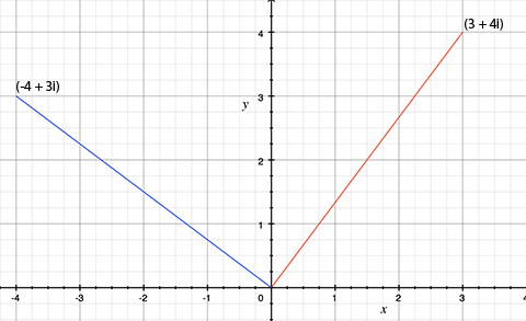
Yep, multiplying by $i$ is a rotation $90^{\circ}$ counter clockwise. So anyways the thing I think is cool, is how it can be represented as a matrix multiply instead of looking like a polynomial multiply.

Identity Operation

The identiy matrix, the matrix that if you multiply by it, it is basically a no-op, why does it act like that, and why is it shaped the way it is? Say you have this matrix multiply:

$\begin{bmatrix} c & 0 \\ 0 & c \end{bmatrix} \cdot \begin{bmatrix} a \\ b \end{bmatrix} = \begin{bmatrix} c \cdot a + 0 \cdot b \\ 0 \cdot a + c \cdot b \end{bmatrix} = \begin{bmatrix} ca \\ cb \end{bmatrix}$

If $c = 1$ then there is your identity operation. But did you ever think:

What are these rows and columns in a matrix really all about?

Say you view that $2x2$ matrix as two unit length column vectors sitting side by side.

$\begin{bmatrix} 1 & 0 \\ 0 & 1 \end{bmatrix}$

The first column $\begin{bmatrix} 1 & 0 \end{bmatrix}^{T}$ and the second column $\begin{bmatrix} 0 & 1 \end{bmatrix}^{T}$ are exactly the basis vectors which define and span $\mathbb{R}^{2}$. Otherwise known as either the x-y or real-imaginary axis.

Change of Basis

So we saw that multiplication by the identity matrix performs no operation at all, because there is just no change to the basis vectors for that space $\mathbb{R}^{2}$. We also saw if we perform a simple change of basis where we scale by $c$, it just scales everything by $c$. The diagonal numbers don’t have to be the same as each other either, if they were different you would get a skewing operation instead of a scaling operation.

$\begin{bmatrix} 2 & 0 \\ 0 & 4 \end{bmatrix} \cdot \begin{bmatrix} a \\ b \end{bmatrix} = \begin{bmatrix} 2 \cdot a + 0 \cdot b \\ 0 \cdot a + 4 \cdot b \end{bmatrix} = \begin{bmatrix} 2a \\ 4b \end{bmatrix}$

Great, so what do the other numbers on the opposite diagonal that have always been $0$ up to this point do? Those numbers let you perform rotations.

Time to Define the $i$ Matrix

If we take the two column matrices we are using as our basis, and rotate them counter clockwise by $90^{\circ}$, which should be easy because they are so simple, we should get the new basis we’re looking for.

$identity = \begin{bmatrix} 1 & 0 \\ 0 & 1 \end{bmatrix} and, \\ i = \begin{bmatrix} 0 & -1 \\ 1 & 0 \end{bmatrix}$

You can see how the first column, instead of being a vector pointing horizontally, is now pointing vertically, and how the second column, which used to, by chance be pointing vertically is now pointing horizontally but in the negative direction, each vector is pointing $90^{\circ}$ counter clockwise to where it used to be pointing.

So what that means, is since we’ve rotated each component $90^{\circ}$ anything vector we multiply by $i$ will also rotate in the same way.

Square Root of Negative One

This should totally be true of a matrix that we decide to name $i$, that is $i^2 = -1$, or well it should equal the matrix version of $-1$.

$\begin{bmatrix} 0 & -1 \\ 1 & 0 \end{bmatrix} \cdot \begin{bmatrix} 0 & -1 \\ 1 & 0 \end{bmatrix} = \begin{bmatrix} -1 & 0 \\ 0 & -1 \end{bmatrix}$

Further proof that this makes any sense:

$\begin{bmatrix} 0 & -1 \\ 1 & 0 \end{bmatrix} \cdot \begin{bmatrix} 3 \\ 4 \end{bmatrix} = \begin{bmatrix} -4 \\ 3 \end{bmatrix}$

Just as the old “graph paper” example predicted. So, I am pretty happy with my explaination of this phenomenon. I have to admit I am just getting used to this Mathjax Latex formatting stuff.

Normally I am happy with a code example, so here is a Ruby example of the same thing:

Ruby example

require 'matrix'

v = Vector[3, 4]

i = Matrix.columns([[0, 1],[-1, 0]])
i * Vector[3, 4]

=> Vector[-4, 3]

i * i
=> Matrix[[-1, 0], [0, -1]]

Other Rotations

We don’t alway want to rotate by $90^{\circ}$, but there is an equation that will let us create a matrix for any arbitrary rotation by $\omega$ radians. And that happens to look like this:

$\begin{bmatrix} cos(\omega) & -sin(\omega) \\ sin(\omega) & cos(\omega) \\ \end{bmatrix}$

Let’s write a Ruby method to create rotation matrices for us, just by passing an angle in radians.

require 'matrix'

def create_rotation_matrix(w)
  sin_w = Math.sin(w)
  cos_w = Math.cos(w)
  Matrix.columns([
      [cos_w,  sin_w],
      [-sin_w, cos_w]]
  )
end

w = Math::PI / 4.0
=> 0.7853981633974483

forty_five = create_rotation_matrix(w)
=> Matrix[[0.7071067811865476, -0.7071067811865475], [0.7071067811865475, 0.7071067811865476]]

v = Vector[3, 4]

forty_five * v
=> Vector[-0.707106781186547, 4.949747468305833]

##  Nice, and rotate by 45 degrees twice?
forty_five * forty_five * v
=> Vector[-3.999999999999999, 3.000000000000001]

##  Now that's a "computer close" type of answer if I ever saw one :)
##  Very close to Vector[-4, 3]

Matrix Form

Now that we’ve established all that stuff about complex numbers and matrices works we sort of have a formula for represeenting a complex number as a matrix.

$3 + 4i = \begin{bmatrix} 3 & -4 \\ 4 & 3 \end{bmatrix}$

So what happens if we use some other sorta pattern besides that? What if we use some other dimension besides the imaginary dimension? What if that dimension was infinitesimal. Most people learn calculus by learning about limits first, but for some reason I didn’t, I learned on my own, and the first calculus textbook that made sense to me taught derivitives using infinitesimals, it’s really similar in some ways, but revolves around the number $\varepsilon$

Derivitives

Derivitives calculate the slope at one point on a curve, when it takes two actual points to calculate a slope, “Rise over Run” style. Usually you see a formula for derivitive using a variable $h$ or $\Delta x$, and take the limit as it goes to 0

$f'(x) = \lim\limits_{\Delta x \to 0} \dfrac{f(x+\Delta x)-f(x)}{\Delta x}$

…but in this “style” of calculus, instead of that, you use $\varepsilon$ where $\varepsilon^{2} = 0$. In math, they say that if there is some positive integer $n$ where $x^n = 0$ then you would call $x$ a nilpotent number

So, example:

$f(x) = x^2 \\ \\ f'(x) = \dfrac{f(x + \varepsilon) - f(x)}{\varepsilon} \\ \\ f'(x) = \dfrac{(x + \varepsilon)^{2} - x^{2}}{\varepsilon} \\ \\ f'(x) = \dfrac{x^{2} + x\varepsilon + x\varepsilon + \varepsilon^{2} - x^{2}}{\varepsilon} \\ \\ f'(x) = \dfrac{2x\varepsilon}{\varepsilon} \\ \\ f'(x) = 2x$

And that all worked out correctly, because $2x$ is totally the derivitive of $x^{2}$. The key to that working out was that we defined $\varepsilon^{2} = 0$, which is something that totally reminds me of defining $i^{2} = -1$.

Dual Numbers

Like a complex number has the form $a + bi$, a dual number has the form $a + b\varepsilon$. The imaginary number $i$ has magic powers, in that it can magically do rotations that you would normally have to use trigonometry for, but a dual number, has the magic power that it can automatically calculate the derivitive of a function.

All you need to do to simultaneously calculate the value of a function, and its derivitive, is pass the function a value of $x + \varepsilon$, that’s whatever $x$ happens to be + $1\varepsilon$.

Simple example again.

$f(x) = x^2 \\ \\ f(x + \varepsilon) = (x + \varepsilon)^{2} \\ \\ f(x + \varepsilon) = x^{2} + x\varepsilon + x\varepsilon + \varepsilon^{2} \\ \\ f(x + \varepsilon) = x^{2} + 2x\varepsilon$

The result of the function is another dual number, the real part of which is $x^{2}$, and the dual part is $2x$, which the value and derivitive at $f(x)$ and $f’(x)$ respectively.

Dual Numbers as Matrices

So just like we can encode a complex number into a 2x2 matrix, we can also encode a dual number in a similar way.

$\varepsilon = \begin{bmatrix} 0 & 1 \\ 0 & 0 \end{bmatrix} \\ \\$

So if we multiply $\varepsilon \cdot \varepsilon$, we should get 0.

$\begin{bmatrix} 0 & 1 \\ 0 & 0 \end{bmatrix} \cdot \begin{bmatrix} 0 & 1 \\ 0 & 0 \end{bmatrix} = \begin{bmatrix} 0 \cdot 0 + 1 \cdot 0 & 0 \cdot 1 + 1 \cdot 0 \\ 0 \cdot 0 + 0 \cdot 0 & 0 \cdot 1 + 0 \cdot 0 \end{bmatrix} = \begin{bmatrix} 0 & 0 \\ 0 & 0 \end{bmatrix}$

Ruby Class for Dual Numbers

####
##  Here is a class that implements Dual numbers, with addition,
##  multiplication, and exponentiation
class Dual
    attr_accessor :matrix
    def initialize(real, dual)
        @matrix = Matrix[[real, dual], [0, real]]
    end
    def +(other)
        result = @matrix + other.matrix
        Dual.new(result[0, 0], result[0, 1])
    end
    def *(other)
        result = @matrix * other.matrix
        Dual.new(result[0, 0], result[0, 1])
    end
    def **(exponent)
        result = @matrix**exponent
        Dual.new(result[0, 0], result[0, 1])
    end
    def to_s
        "#{real} + #{dual}ε"
    end
    def inspect
        to_s
    end
    def real
        @matrix[0, 0]
    end
    def dual
        @matrix[0, 1]
    end
end
#
####
##  Now let's have f(x) = x**2
def f(x)
    x**2
end
####
##  Let's print a few values of this function
print "f(x) = "
p (0..15).map{|x| f(x) }
## This prints:
## f(x) = [0, 1, 4, 9, 16, 25, 36, 49, 64, 81, 100, 121, 144, 169, 196, 225]
#  
#  
####
##  Now lets run function f on a dual number, f(x + ε)
print "f(x + ε) = "
p (0..15).map{|x| f(Dual.new(x, 1)) }
# 
# 
##  This prints
##  f(x + ε) = [0 + 0ε, 1 + 2ε, 4 + 4ε, 9 + 6ε, 16 + 8ε, 25 + 10ε, 36 + 12ε, 
##              49 + 14ε, 64 + 16ε, 81 + 18ε, 100 + 20ε, 121 + 22ε, 144 + 24ε, 
##              169 + 26ε, 196 + 28ε, 225 + 30ε]
# 
# 
##  The real part of the dual number in f(x + ε) is exactly the same as f(x)
##  Let's just print out the dual component instead
# 
print "Dual{f(x + ε)} = "
p (0..15).map{|x| f(Dual.new(x, 1)).dual }
# 
# 
##  This prints
##  Dual{f(x + ε)} = [0, 2, 4, 6, 8, 10, 12, 14, 16, 18, 20, 22, 24, 26, 28, 30]

Conclusion

I dunno, thought that was pretty cool. Actually the more I figure out about matrices the more I am understanding how they can be used to implement any linear operator. Actually the reasoning behind me even caring about matrices or linear operators at all (or math really), is that works together well with my obsession for digital audio filters. Because a digital filter is usually a linear operation, yep, matrices can be used to calculate filters :) Hopefully I will get more into describing how filters work in future blog posts.